How to Build Semantic Search with Embeddings: a Practical Walkthrough

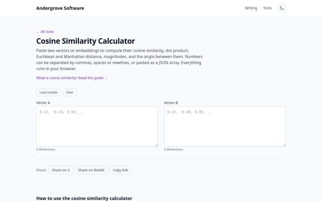
The pipeline in one paragraph

Split your documents into chunks, turn each chunk into an embedding vector once and store the vectors. At query time, embed the user’s question with the same model, score it against every stored vector with cosine similarity, and return the top-scoring chunks. That is the entire architecture; everything else — vector databases, hybrid ranking, re-rankers — is optimization layered on top. (If embeddings themselves are new to you, start with embeddings and cosine similarity explained.)

Step 1: chunk your documents

Embedding whole documents produces mushy averages — a 40-page manual embedded as one vector is "about" everything and matches nothing well. Split into chunks of roughly 200–500 tokens, aligned to natural boundaries (headings, paragraphs) with a little overlap so ideas straddling a boundary survive. Chunk size is the single most consequential tuning choice: small chunks give precise matches with little context, large ones the reverse. The text chunker lets you preview exactly how a document splits before you commit.

Step 2: embed the chunks

Run every chunk through an embedding model — via an API or a local sentence-transformer — and store the returned float vectors alongside the chunk text. Two rules are non-negotiable: use the same model for documents and queries (vectors from different models live in unrelated spaces, so their similarities are meaningless), and re-embed everything if you ever switch models. This step costs the most compute, but it runs once per document, not per query.

Step 3: rank with cosine similarity

With vectors in hand, search is a normalize-once dot product:

import numpy as np

# docs: (n_chunks, dim) matrix, embedded once
docs = docs / np.linalg.norm(docs, axis=1, keepdims=True)

def search(query_vec, k=5):
    q = query_vec / np.linalg.norm(query_vec)
    scores = docs @ q                # cosine similarity, all chunks at once
    top = np.argsort(-scores)[:k]
    return [(int(i), float(scores[i])) for i in top]

Normalizing rows up front turns every later cosine into a plain dot product, and the matrix multiply scores all chunks in one shot.

Do you need a vector database?

Later than you think. Brute-force numpy over 100,000 vectors answers in milliseconds on a laptop — for a personal knowledge base, documentation site or small product, an array in memory is the whole system. Reach for a vector database when you have millions of vectors, need metadata filtering combined with similarity, or documents change constantly. Starting with numpy also gives you a correctness baseline to test the fancier index against.

Tuning: thresholds, hybrid search, evaluation

Absolute scores vary by model, so never hard-code a "good" threshold from folklore — rank first, then add a floor tuned on your own data to suppress garbage matches when nothing relevant exists. Pure semantic search is also weak on exact identifiers (part numbers, error codes, names), so production systems usually blend a keyword score with the cosine score — "hybrid search". Before tuning anything, build a tiny evaluation set of 20–30 real queries with known best chunks and check how often the right one lands in the top 3; it turns guesswork into measurement. To debug surprising matches, paste the two texts into the calculator and inspect the score directly, or project your whole corpus visually with the embedding projector.

Ready to try it? Open the Cosine Similarity Calculator →